Reproducing figures from squidpy manuscript
Source:vignettes/C_reproduceSquidpyFigures.Rmd
C_reproduceSquidpyFigures.RmdIntroduction
This vignette will demonsrate to the user how to reproduce some figures from the Squidpy manuscript. The authors of squpidpy documented their work via a Jupyter notebook that we then translated into R code. The steps below use the R package reticulate to translate python code into R code that then create figures from the manuscript. Reticulate makes it very easy to use python code within R with very few changes. We will do a couple comparisons between python code and the reticulate R code to demonstrate where changes may have to be made.
Set up
Import python packages
Reticulate has a very convenient function for importing the python libraries needed to perform certain tasks. It is important to note that the environment where squidpy was installed should be active in order for this code to work.
For examples, I named my conda environment squidpy so I’ll run
conda activate squidpy before running the follow code in
R.
Settings
There are some setting that are set in the Jupyter notebook that can
be done here as well. When converting python code to R code any
. will become a $. The first code chunk is a
python code chunk and then the following code chunk would be the
corresponding R code. Some settings did not translate so I will comment
them out in the python code.
Python code
sc.logging.print_header()
#> scanpy==1.9.3 anndata==0.9.1 umap==0.5.3 numpy==1.22.4 scipy==1.9.1 pandas==2.0.1 scikit-learn==1.2.2 statsmodels==0.13.5 python-igraph==0.10.4 pynndescent==0.5.10
sc.set_figure_params(facecolor="white", figsize=(8, 8))
sc.settings.verbosity = 3
#sc.settings.dpi = 300
#sq.__version__
sc.settings.figdir = "./figures"
R code
sc$logging$print_header()
sc$set_figure_params(facecolor="white", figsize = c(8,8))
sc$settings$verbosity = 'hint'
sc$settings$figdir = "./figures"

PATH_FIGURES = "./figures"
Obtain data
The data used is provided as part of the squpidpy package. We load it into R with the following code, note that is is an anndata object.
adata <- sq$datasets$seqfish()
adata # 19416 obs x 351 vars
#> AnnData object with n_obs × n_vars = 19416 × 351
#>     obs: 'Area', 'celltype_mapped_refined'
#>     uns: 'celltype_mapped_refined_colors'
#>     obsm: 'X_umap', 'spatial'
Figures
For the rest of this vignette we will be following the Jupyter notebook and translating the python code to R. Each plot is created and saved in the figures directory for future use.
Figure 1
sc$pl$spatial(
    adata,
    color = "celltype_mapped_refined",
    save = "_seqfish.png",
    spot_size = 0.03
)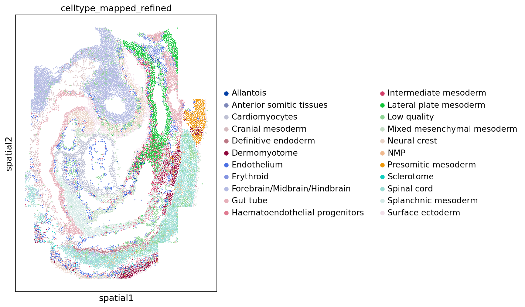
Figure 1
Figure 2
For this figure we will show the python code and the corresponding R code to demonstrate where there may be some differences.
sq.gr.spatial_neighbors(adata, delaunay=True)
#> Creating graph using `generic` coordinates and `None` transform and `1` libraries.
#> Adding `adata.obsp['spatial_connectivities']`
#>        `adata.obsp['spatial_distances']`
#>        `adata.uns['spatial_neighbors']`
#> Finish (0:00:02)
sq.gr.nhood_enrichment(adata, cluster_key="celltype_mapped_refined", n_perms=1000)
#> Calculating neighborhood enrichment using `1` core(s)
#>
  0%|          | 0/1000 [00:00<?, ?/s]
  3%|3         | 30/1000 [00:00<00:03, 299.50/s]
 10%|9         | 97/1000 [00:00<00:01, 514.15/s]
 16%|#6        | 163/1000 [00:00<00:01, 578.12/s]
 23%|##2       | 229/1000 [00:00<00:01, 609.83/s]
 30%|##9       | 296/1000 [00:00<00:01, 625.64/s]
 36%|###6      | 363/1000 [00:00<00:00, 638.33/s]
 43%|####2     | 429/1000 [00:00<00:00, 642.64/s]
 50%|####9     | 496/1000 [00:00<00:00, 650.95/s]
 56%|#####6    | 564/1000 [00:00<00:00, 659.02/s]
 63%|######3   | 632/1000 [00:01<00:00, 663.32/s]
 70%|#######   | 702/1000 [00:01<00:00, 671.87/s]
 77%|#######7  | 770/1000 [00:01<00:00, 673.80/s]
 84%|########3 | 838/1000 [00:01<00:00, 666.53/s]
 91%|######### | 908/1000 [00:01<00:00, 673.97/s]
 98%|#########8| 980/1000 [00:01<00:00, 687.31/s]
100%|##########| 1000/1000 [00:01<00:00, 646.21/s]
#> Adding `adata.uns['celltype_mapped_refined_nhood_enrichment']`
#> Finish (0:00:01)
arr = np.array(adata.uns["celltype_mapped_refined_nhood_enrichment"]["zscore"])

sq.pl.nhood_enrichment(
    adata,
    cluster_key="celltype_mapped_refined",
    cmap="coolwarm",
    title="",
    method="ward",
    dpi=300,
    figsize=(5, 4),
    save="nhod_seqfish.png",
    cbar_kwargs={"label": "Z-score"},
    vmin=-50,
    vmax=50,
)
sq$gr$spatial_neighbors(adata, delaunay = TRUE) # added to adata.obsp, adata.uns
sq$gr$nhood_enrichment(adata, cluster_key = "celltype_mapped_refined", n_perms = 100) # added to adata.uns

arr <- np$array(adata$uns["celltype_mapped_refined_nhood_enrichment"]["zscore"])

sq$pl$nhood_enrichment(
    adata,
    cluster_key = "celltype_mapped_refined",
    cmap = "coolwarm",
    title = "",
    method = "ward",
    dpi = 300,
    figsize = c(5, 4),
    save = "nhood_seqfish.png",
    cbar_kwargs = list(label = "Z-score"),
    vmin = -50,
    vmax = 50
)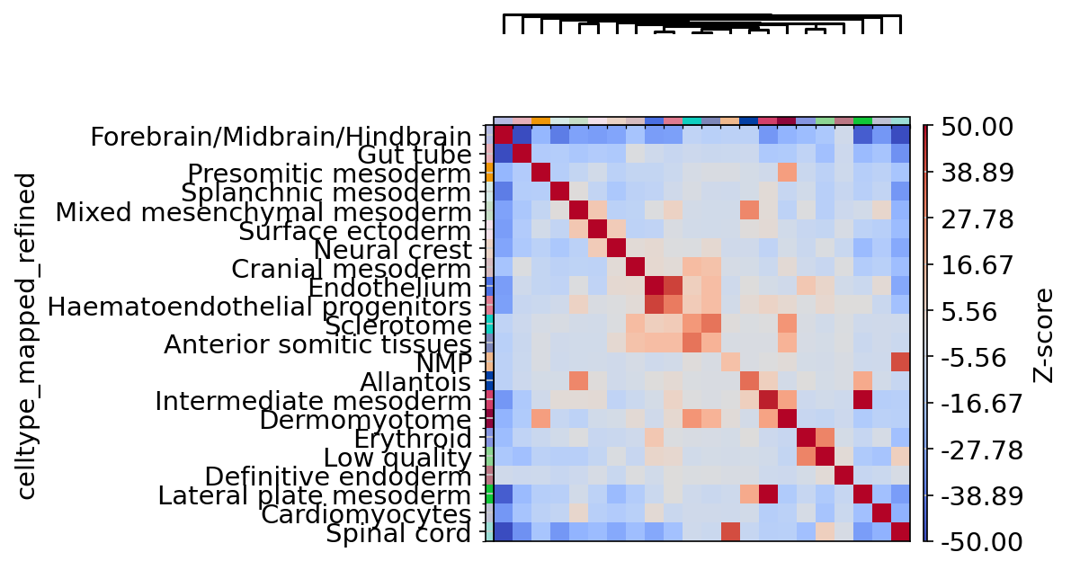
Figure 2
Figure 3
sq$pl$nhood_enrichment(
    adata,
    cluster_key = "celltype_mapped_refined",
    cmap = "inferno",
    title = "",
    method = "ward",
    dpi = 300,
    figsize = c(5, 4),
    save = "nhod_seqfish.png",
    cbar_kwargs = list(label = "Z-score"),
    vmin = -50,
    vmax = 150
)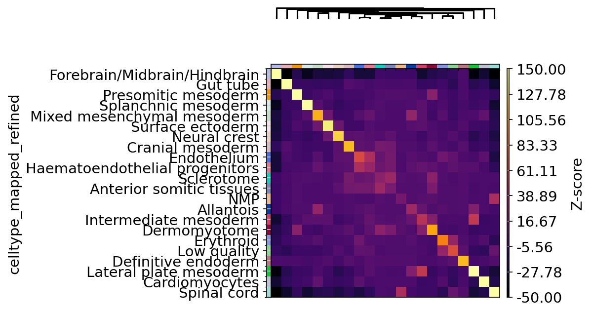
Figure 3
Figure 4
ax <- plt$subplots(
    figsize = c(3, 6)
)
sc$pl$spatial(
    adata,
    color = "celltype_mapped_refined",
    groups = c(
        "Endothelium",
        "Haematoendothelial progenitors",
        "Allantois",
        "Lateral plate mesoderm",
        "Intermediate mesoderm",
        "Presomitic mesoderm",
        "Dermomyotome"
    ),
    save = "_endo_seqfish.png",
    frameon = FALSE,
#    ax = ax,
    show = FALSE,
    spot_size = 0.03
)
#> [[1]]
#> <Axes: title={'center': 'celltype_mapped_refined'}, xlabel='spatial1', ylabel='spatial2'>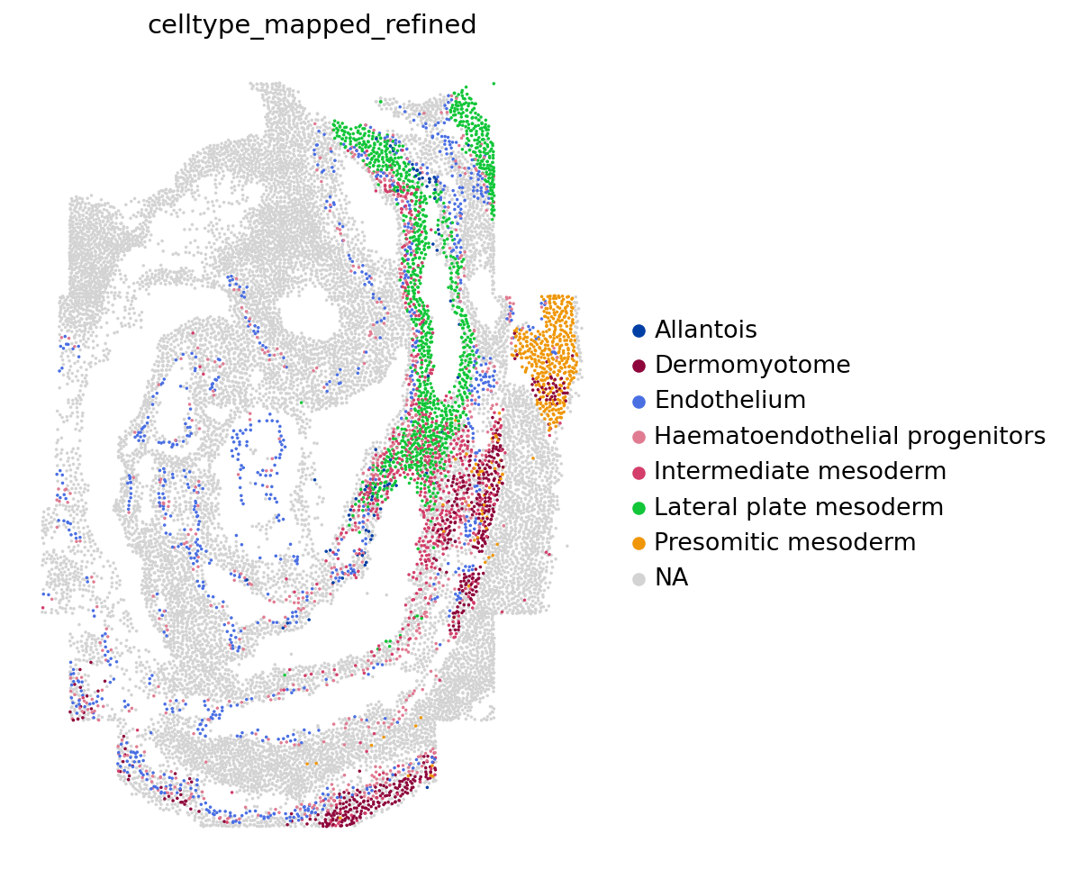
Figure 4
Figure 5
sc$pl$spatial(
    adata,
    color = "celltype_mapped_refined",
    groups = c(
        "Allantois",
        "Lateral plate mesoderm",
        "Intermediate mesoderm",
        "Presomitic mesoderm"
    ),
    save = "_meso_seqfish.png",
    spot_size = 0.03,
#    ax = ax,
    show = FALSE
)
#> [[1]]
#> <Axes: title={'center': 'celltype_mapped_refined'}, xlabel='spatial1', ylabel='spatial2'>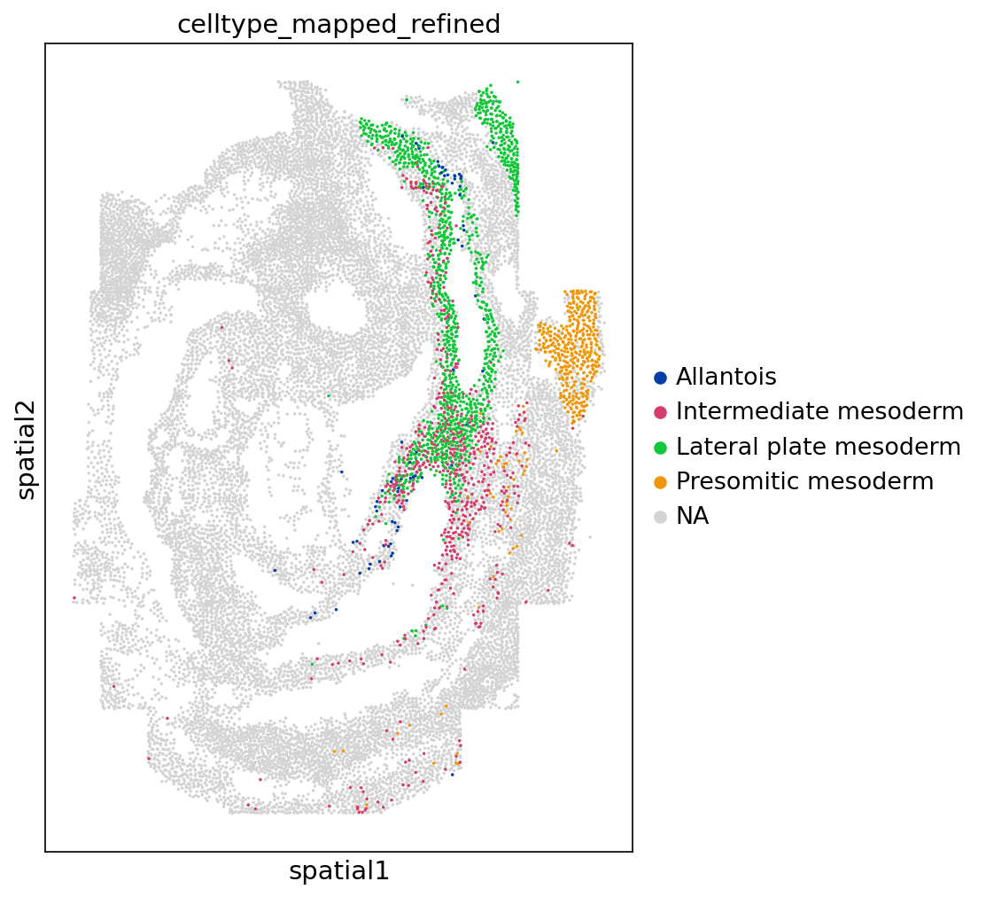
Figure 5
Figure 6
sq$gr$co_occurrence(
    adata,
    cluster_key = "celltype_mapped_refined"
) # added to adata.uns


sq$pl$co_occurrence(
    adata,
    cluster_key = "celltype_mapped_refined",
    clusters = "Lateral plate mesoderm",
    figsize = c(5, 3),
    legend = FALSE,
    dpi = 300,
    save = "co_occurrence_seqfish"
)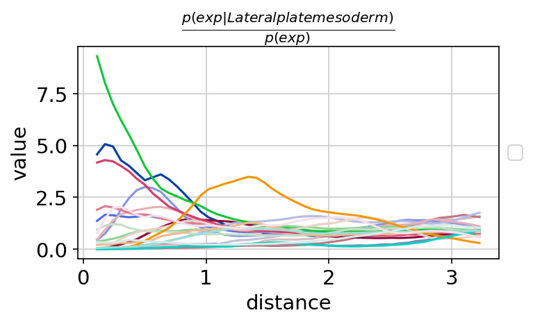
Figure 6